Tutorials
These tutorials explain in each details how each scripts works and how to use them to study a corpus of bibliographic data. To summarize:
| biblio_parser.py | ⇒ pre-processes WOS / Scopus data files, |
| corpus_description.py | ⇒ performs a frequency analysis of the items in corpus, |
| filter.py | ⇒ filters the corpus according to a range of potential queries, |
| biblio_coupling.py | ⇒ performs a BC anaysis of the corpus, |
| cooc_graphs.py | ⇒ produces various co-occurrence graphs based on the corpus, |
| all_in_one.py | ⇒ launches all these analyses on a series of temporal slices of the corpus. |
Don't forget to check that all necessary python package are installed on your system (cf the list on the Download page). To be able to use the BiblioMaps visualisation interface, you'll also need to have a localhost set up on your system. Here's a link to webpage explaining how to set up a local web server on most OS.
Create project folders
The "BiblioTools3.2" folder containing the python scripts can be stored anywhere on your computer, the easiest place being your desktop if you intend to use it often. Before starting a new project, you'll also need to create
- a folder that will contain the raw bibliographic files as well as all the intermediate data files generated by BiblioTools. I'll assume in these tutorials that a "MY_PROJECT_NAME" folder was created on your Desktop, with a subfolder name "rawdata".
- a copy of the "BIBLIOMAPS_myprojectname" folder in your localhost repository.
Data extraction
From the WEB OF SCIENCE
The Web Of Science (WOS) is one of the most comprehensive bibliographic database, providing extensive and well-formatted bibliographic publication records. It does however suffer from a relatively low coverage of social sciences and of publications sources written in non-english languages.
Depending on your project, you might want to collect records of publications using a given set of keywords / references / authors / institutions / publications journals, etc. For example, you may use the Advanced search interface to write a query based on various names of an institution such as AD="Ecole Normale Super Lyon" OR AD="ENS LYON" OR AD="ENS de Lyon" to extract records from publications written by researchers from a given institution (here, the ENS Lyon).
To extract bibliographic data, use the "Output records" menu of the "Results" page:
- select the publications whose records you want to extract (you can only download 500 records at a time)
- select "Full Records + Cited References" as the output format
- save the records in a "tab-delimited" format (either "win" or "mac") with UTF-8 encoding (this is crucial to avoid encoding issues later).
When you are done downloading all the records, move all the extracted "savedrecs" .txt files within your "rawdata" project folder.
From SCOPUS
Scopus is another one of the most comprehensive bibliographic database, providing well-formatted bibliographic records. Scopus does also suffer from a relative lack of coverage in social sciences / non-english publications.
While WOS and Scopus share a core of indexed publications sources, they also both cover publication sources that are not indexed in their concurrent database. Depending on the disciplinary nature of the corpus you want to extract, it may thus be more relevant to use one or the other.
Use one of the available interface (eg the Advanced search one) to type a query and select a corpus. To extract bibliographic data, go on the result page and
- use the Refining options ("Limit to" and "Exclude") to select a subpart of the publications whose records you want to extract (you can only download 2000 records at a time)
- select "All" documents
- "export" them, choosing the csv output format and selecting all information types (citation informmation, bibliographical information, abstract & keywords, funding details, other information)
When you are done downloading all the records, move all the extracted "scopus" .csv files within your "rawdata" project folder.
Can I merge data extracted from WOS and SCOPUS in a single project? While it could be done, BiblioTools does not allow you to do that, the reason being that WOS and SCOPUS formatting have significant differences (in the way references are formatted, in publications sources' abbreviations, in their generated keywords and categories, in the number of citation they record, etc). Furthermore, about only 80% of the documents in WOS or SCOPUS have a DOI (standard document identifier), cf this source. Hence, merging data extracted from WOS and SCOPUS would result in duplicate problems and matching problems (between various ways to refer to a journal, a conference, an institution, a reference, etc). Avoid this mess!
How large a corpus can the BiblioTools handle? All the codes should run rather smoothly on a simple laptop for up to 150,000-200,000 publications corpora - you'll get memory problem with larger ones.
Data parsing
Before doing any analysis, the WOS or Scopus files need to be pre-processed in order to store the different bibliographic entities (authors, keywords, references, etc) into more manageable data files. This task is performed by the "biblio_parser.py" script. To execute this scrpt, open your terminal, cd to your Desktop and simply execute the following command line:
The options -i and -o indicate the data input and output folders. The option -d indicates the orgin of the data to parse (either "-d wos" or "-d scopus", wos being the default option).
The script produces a series of data files:
- articles.dat is the central file, listing all the publications within the corpus. It contains informations such as the document type (article, letter, review, conf proceeding, etc), title, year of publication, publication source, doi, number of citations (given by WOS or Scopus at the time of the extraction) AND a unique identifier used in all the other files to identify a precise publication.
- database.dat keeps track of the origin of the data, some part of the analysis being specific to WOS or Scopus data.
- authors.dat lists all authors names associated to all publications ID.
- addresses.dat lists all adresses associated to all publications ID, along with a specific ID for each adresse line. These adresses are reported as they appear in the raw data, without any further processing.
- countries.dat lists all countries associated to all publications ID and adresses lines ID. The countries are extracted from the adresses fields of the raw data, with some cleaning (changing mentions of US states and UK countries to respectively the USA and UK).
- institutions.dat lists all the comma-separated entities appearing in the adresses field associated to all publications ID and adresses lines ID, except those refering to a physical adresses. These entities correspond to various name variants of universities, organisms, hospitals, labs, services, departments, etc as they appear in the raw data. No treatment is made to e.g. filtering out the entities corresponding a given hierarchy level.
- keywords.dat lists various types of keywords associated to all publications ID. "AK" keywords correspond to Author's keywords. "IK" keywords correspond to either WOS or Scopus keywords, which are built based on the authors' keywords, the title and abstract. "TK" correspond to title words (from which we simply remove common words and stop words - no stemming is performed). TK are especially useful when studying pre-90's publications, when the use of keywords was not yet standard.
- references.dat lists all the references associated to all publications ID. The rawdata is parsed to store the first author name, title, source, volume and page of each reference of the raw "references" field.
- subjects.dat lists all subject categories associated to all publications ID (a journal may be associated to many subject category). WOS classifies the sources it indexes into ∼ 250 categories, that are reported in the extracted data. Scopus classifies its sources into 27 major categories and ∼ 300 sub-categories, none of which are reported in the extracted data. We use Elsevier Source Title List (october 2017 version) to retrieve that information. The "subject.dat" contains the info relative to the major categories.
- subjects2.dat lists Scopus's sub-categories, if the use database is Scopus.
- AA_log.txt keeps track of the date/time the script was executed and of all the messages displayed on the terminal (number of publications extracted, % of references rejected, etc).
An expert mode is also available: adding the option "-e" in the command line above, complementary files will be generated:
- AUaddresses.dat (WOS only) lists all linked (authors, adresses) associated to all publications ID, when this information is available (we almost always have the authors and addresses info, but not always the "this address correspond to this author" info).
- abstracts.dat lists the abstracts associated to all publications ID. This file is not generated in the normal mode to avoid unecessary memory occupation.
- cities.dat lists all cities associated to all publications ID and adresses lines ID. The cities are extracted from the adresses fields of the raw data, with some cleaning (zip codes removed).
- fundingtext.dat (WOS only) lists the funding text associated with all publications ID.
The script does not work and is unterrupted mid-course, why is that happening? Some indications of the problem should appear on the terminal console. Most often, the problem comes from a bad formatting of an extracted file, which may have been extracted in the wrong format or corrupted during the upload (e.g. the end of the file is missing, or it is written in a binary format). In that case, you just have to identify this file and re-upload the corresponding data. If you can't solve your problem, you can always try to shoot me an email, with a link to your rawdata and a screenshot of the logs appearing in the console!
Corpus description
Analysing the data
Before doing anything else, you should get a general idea of the content of your database. Execute the following command line:
The options -i indicates the data input folder and the option -v puts the verbose mode on (detailed info about the script process will be displayed in the terminal). This script performs several basic tasks:
- it performs a series of frequency analysis, computing the number of occurrences of each item (authors, keywords, references, etc) within the publications of the corpus. These frequencies are automatically stored into several "freq_xxx.dat" files within a newly created "freq" folder.
- it performs a series of generic statistical analysis, storing the numbers of distinct items of each type (e.g. there are x distinct keyword in the corpus ), the distributions of number of occurrences of each item (e.g. there are x keywords appearing in at least y publications) and the distribution of number of items per publication (e.g.there are x% of publications with y keywords). All these statistics are stored in the "DISTRIBS_itemuse.json" file.
- it also performs a co-occurrence analysis, computing the number of co-occurrence of pairs of items among the top 100 most frequent items of each type (e.g. computing how often the two most used keywords appear together in the same publications). The results of this analysis are stored in the "coocnetworks.json" file. More systematic co-occurrence analysis can also be performed with another script, cf the Co-occurrence Maps section below.
All the generated files can be opened and read with a simple text editor. The freq_xxx.dat, listing items by order of frequency, can also be read in a spreadsheet software such as excel. All the files are however primarily made to be read in the BiblioMaps interface.
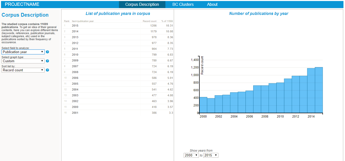
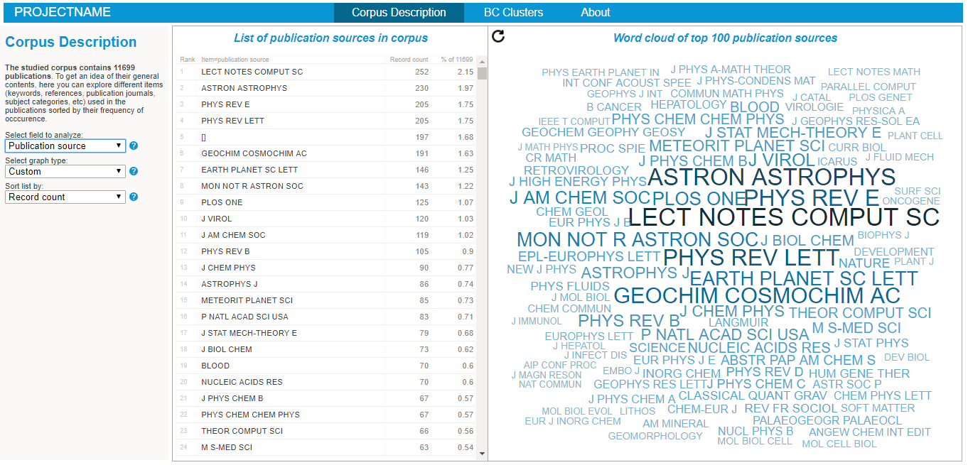
Exploring the nature of the corpus in the BiblioMaps interface
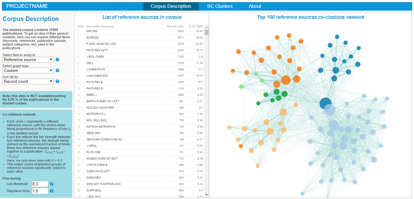
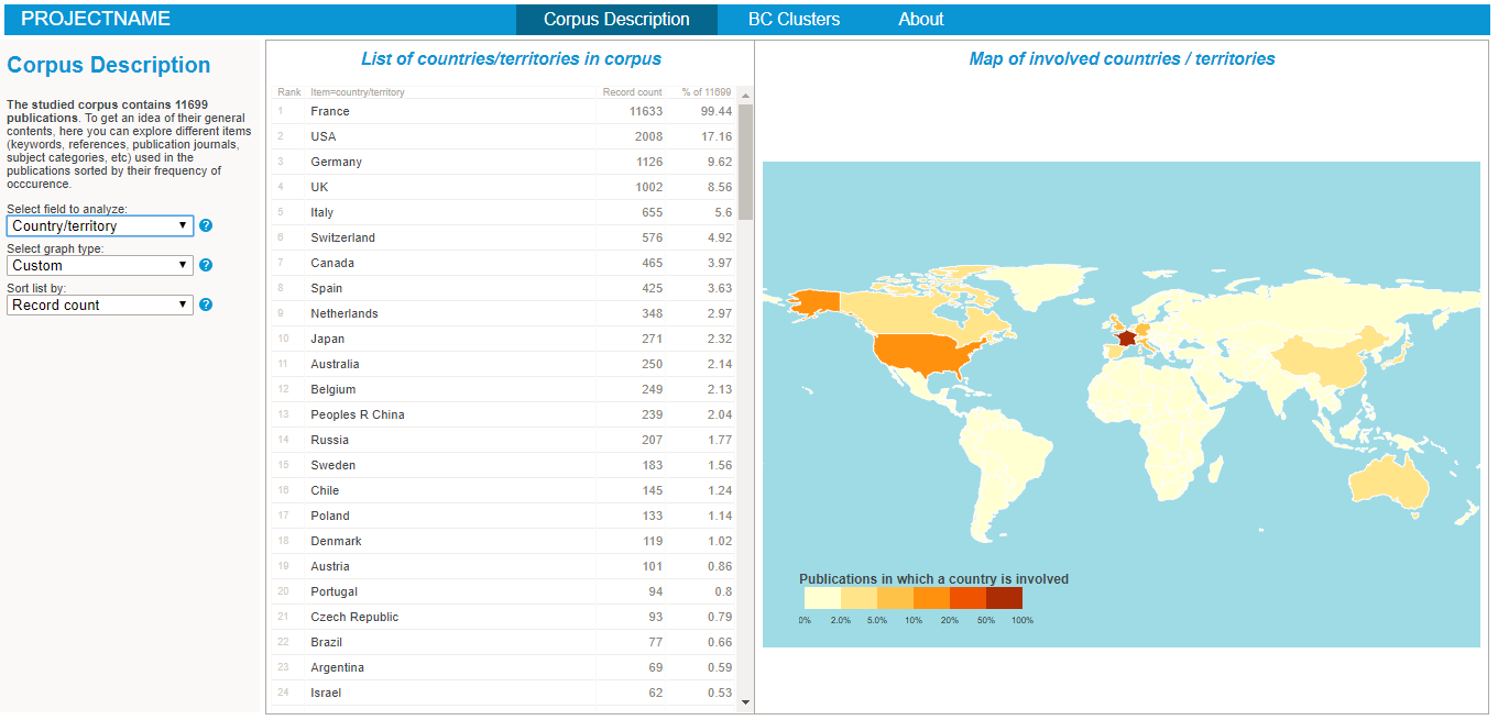
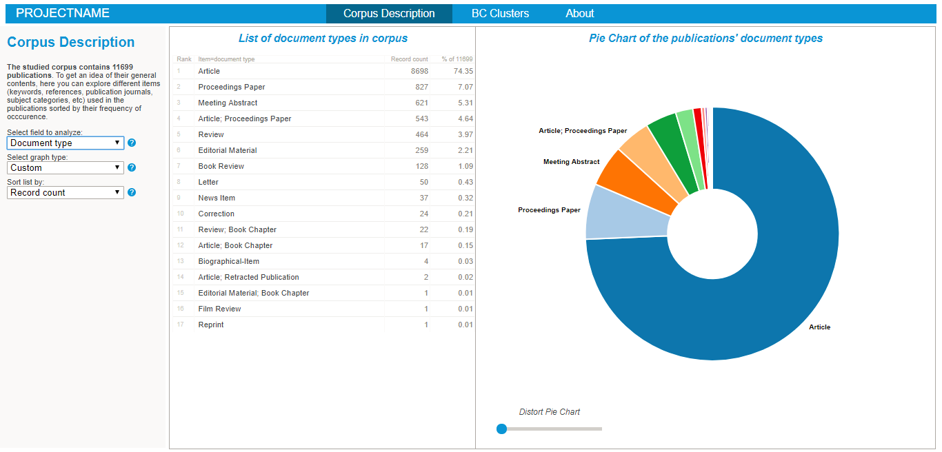
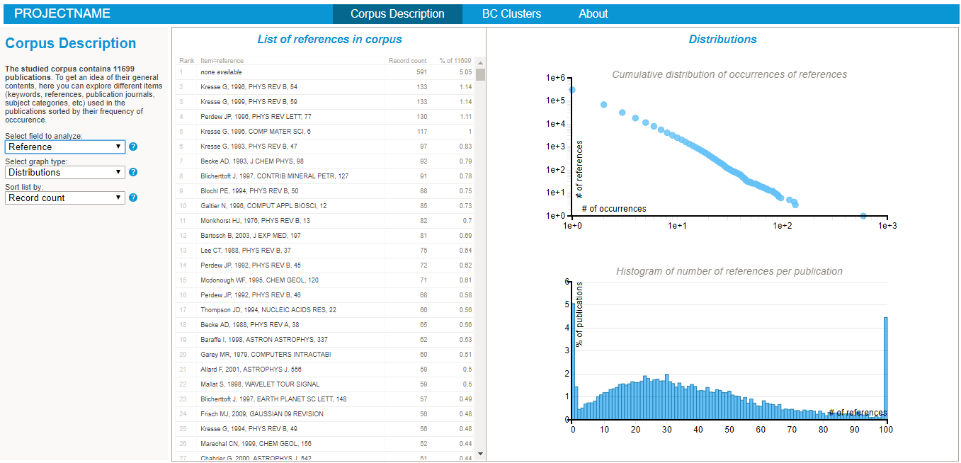
To start explore the nature of your corpus, simply:
- Cut-paste the "freq" folder from "myprojectname" to the "BIBLIOMAPS_myprojectname/data" folder in your localhost repository.
- Open your browser (preferably chrome or firefox), go to localhost/[path_to_BIBLIOMAPS_myprojectname]/corpus.html
- Explore the various lists and visualisations (cf examples on the right hand side)!
- Use the controls at the bottom left of the interface to fine-tune the link threshold and the repulsive force used in the layout algorithm.
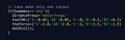
- Once you have selected values you are OK with, you may want to set them at default values. Open the "corpus.html" file and edit the "fooTHR" and "fooForce" dictionnaries on line 103 (cf last figure on the diaporama). The labels 'K', 'AK', 'TK', 'S', R' and 'RJ' used in the dictionnaries respectively refer to the keywords, authors' keywords, title words, subject categories, reference and references sources co-occurrence networks.
Some incoherent items are displayed on the lists, how comes? There might occassionaly be some manual cleaning to do in the "freq_xxx.dat" files. In particuler, if you used data extracted from Scopus, you may want to delete some lines corresponding to wrong items in the "language", "doctype" and "countries" files.
I can spot a same reference appearing twice or more in the reference list, with only a small difference in the way it is written. Why not systematically group them together? Despite WOS / Scopus huge work of normalisation of the references, some references may indeed appear under several small variant (first author names with or without middle name initial, book title with or without its subtitle, publication source abbreviated or not, different editions of a book with diffferent publication years may exist, etc). So what should we do about that? Option 1: leave the data as it is, and you may have to take into account potential effect in the subsequent analysis (e.g. in the BC analysis, you may see a separation between two communities of researchers citing two distinct editions of a same book, which could be interesting). Option 2: manually clean-up the "references.dat" file, at least for a few important references, and re-do all the previous steps.
I have done some changes in the data file but can't see them in the BiblioMaps interface. Try to clear your browser's stored data, and refresh.
Filtering the data
If, upon exploring the nature of the data you realize that before going further you'd prefer to filter your corpus based on some characteristic (keeping only the publications from certain years, using some keywords or references, written by some authors from some countries, etc), you can filter the initial corpus thanks to the script:
Edit the 'filter.py' file to specify your filters. You'll also need to create a new "myprojectname_filtered" main folder before running the script.
Bibliographic Coupling Maps
Methodology
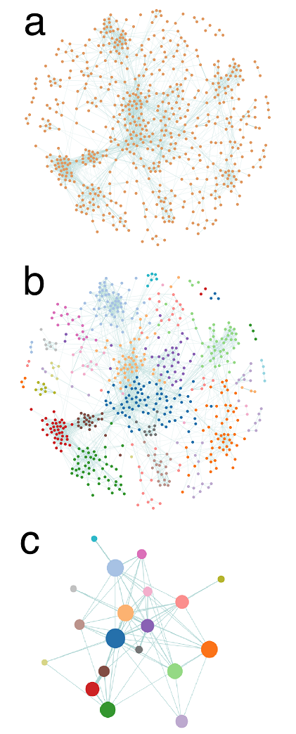
Cluster detection on a BC network of ∼ 600 publications.
Network construction: bibliographic coupling (BC) is based on the degree of overlap between the references of each pair of publications. Specifically, BC is performed by computing Kessler' similarity between publications: ωij=Rij/√(RiRj), where Rij is the number of shared references between publications i and j and Ri is the number of references of publication i. If two publications do not share any reference, they are not linked; if they have identical references, the strength of their connexion is maximal. On Fig. a, each node represents a publication, and the thickness of a link is proportional to the similarity between two publications. On this figure and the next, the layouts are determined by a force-based spatialisation algorithm (ensuring that strongly linked nodes are closer to each other).
Cluster detection: a community detection algorithm based on modularity optimization (we use an implementation of the Louvain algorithm) is applied to partition the publications into clusters. Basically, the algorithm groups publications belonging to the same "dense" - in terms of links - region of the BC network, cf Fig. b.
Cluster representation: publications belonging to the same cluster are gathered into a single node, or circle, whose size is proportional to the number of publications it contains, cf Fig. c. A standard frequency analysis is then performed to characterise each cluster with its more frequent / significant items (keywords, references, authors, etc), which can then be used as automatic labels.
Hierarchical clustering: the exact same methodology can be applied to the subsets of publications belonging to each detected cluster to split them into sub-clusters.
What are the advantages of BC analysis? Compared to what happen in co-citation analysis (the other main bibliographic technique, linking publications that are cit.ed together in other publications), the membership of a given publication in this or that cluster is immediate: it is determined by the references used by the authors and does not depend on how the publication will be cited later. In that respect, BC is - among other things - a relevant technique to detect emerging communities.
Bibliographic Coupling analysis
You may execute the bibliographic coupling script with the command line:
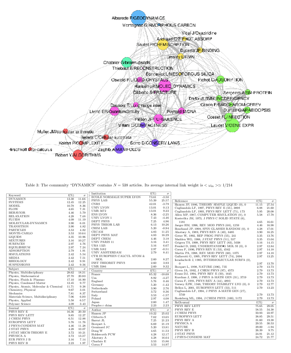
Example of BC clusters network visualisation created in Gephi and of one cluster's ID card, part of a lengthy PDF document listing the ID cards of all clusters.
The options -i indicates the data input folder and the option -v puts the verbose mode on. This script execute a number of tasks:
- It first creates the BC network, computing Kessler similarities between each pair of publications
- It detects a first set of clusters (which we will refer to as "TOP") using Thomas Aynaud's python implementation of the louvain algorithm. A second set of clusters ("SUBTOP") is then computed by applying the same algorithm to the publications in each TOP cluster, hence providing a 2-level hierarchical partition.
- The script will then asked whether you want to create output files for the cluster. By default, the script will output information only for clusters with more than 50 publications, but the script will asked you to confirm / change this threshold. Several files will then be created by the script:
- Output 1: two json files, storing information about the clusters, to be used in the BiblioMaps interface (cf below).
- Output 2a: two .tex files (one for each hierarchical level) you'll have to compile, displaying an "ID Card" for each cluster, ie the list of the most frequent keywords, subject, authors, references, etc... used by the publications within this cluster.
- Output 2b: one .gdf file storing information relative to the BC clusters at both the TOP and SUBTOP level. You may open this file with Gephi. You may create visualisations of either the TOP or SUBTOP level by filtering it out, resie the nodes with the "size" parameter, run a spatialisation layout algorithm (Force Atlas 2 usually yield satisfaying layouts). You may also choose a label within the few that are available (e.g. 'most_frequent_k' correspond to the most frequent keywords of each cluster). Refer to the Id cards created with latex to know more about the content of each cluster.
- Finally, the script proposes you to output the BC network at the publication level, in both a gdf output format that can be opened with Gephi and a json format that can be opened in the BiblioMaps interface. You may either keep the whole network or select only the publications within a given cluster. Keep in mind that both interfaces can only handle a given number of nodes (no more than a few thousands for Gephi, a few hundreds for BiblioMaps).
Fine-tuning the BC methodology. At the very beginning of the "biblio_coupling.py" script, you may edit a few parameters used in the definition if the BC network. For example, edit the parameter "bcthr" is you want to restrain the creation of a BC link to pairs of publications sharing at least "bcthr" references (default value is set to 1) or edit the parameter "DYthr" if you want to restrain the creation of a BC link to pairs of publications published less than DYthr years appart (default is 10000 years). The names of the files created when changing the default values of these parameters will contain suffixes reflecting these changes (eg "BCclusters_thr2.json"). To open these generated files in the BiblioMaps interface, you'll have to edit the "defaultfile" and "datafile" parameters in "BCclusters.html" (at about line 195).
How can I open the "BCpublis.json" file, storing the BC network at the publication level, in BiblioMaps? Cut/paste the json file in the "BIBLIOMAPS_myprojectname/data" folder in your localhost repository and uncomment the link to the "BCpublis.html" tab in the "headermenu.html" file. Refresh your webpage (you may need to clear your browser's stored data) and voilà!
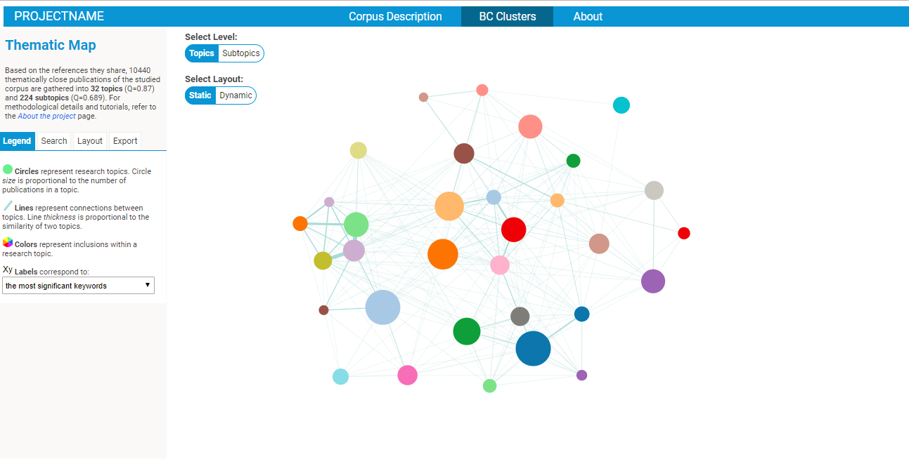
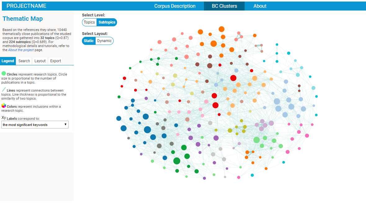
Exploring BC clusters in the BiblioMaps interface
To start explore the nature of your corpus, simply:
- Cut-paste the two files within the "json" folder from "myprojectname" to the "BIBLIOMAPS_myprojectname/data" folder in your localhost repository.
- Open your browser (preferably chrome or firefox), go to localhost/[path_to_BIBLIOMAPS_myprojectname]/BCclusters.html
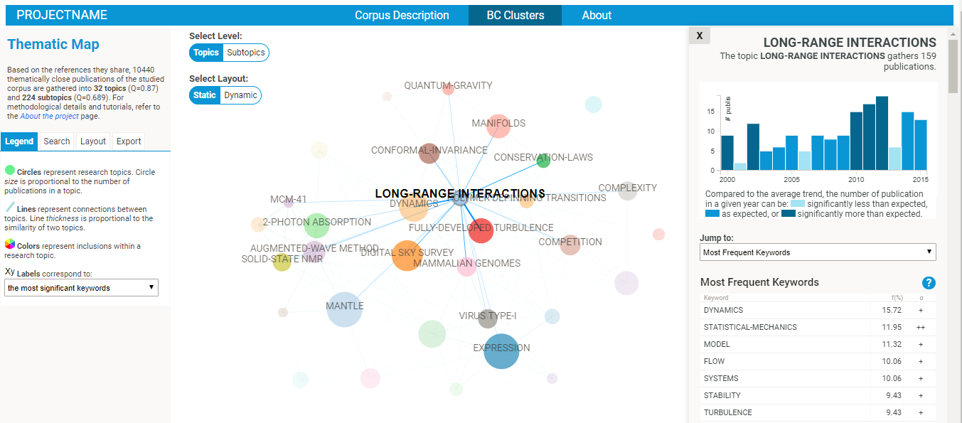
- Explore the BC network! Several intuitive functionalities will allow you to :
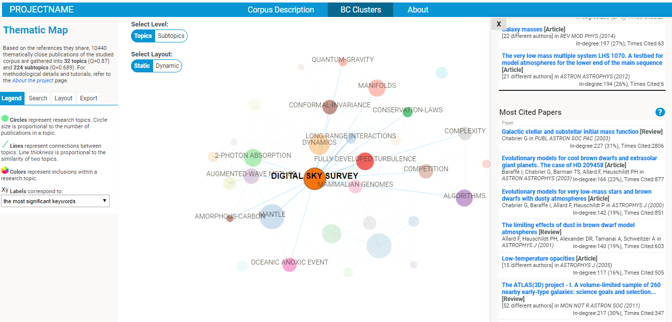
- explore the nature of each cluster (in terms of most frequent references, publication sources, subject categories, keywords, etc).
- google scholar search links are provided for the most cited papers and authors of each cluster, so that you might easily find a full text publication.
- you may change the label of the cluster according to several options
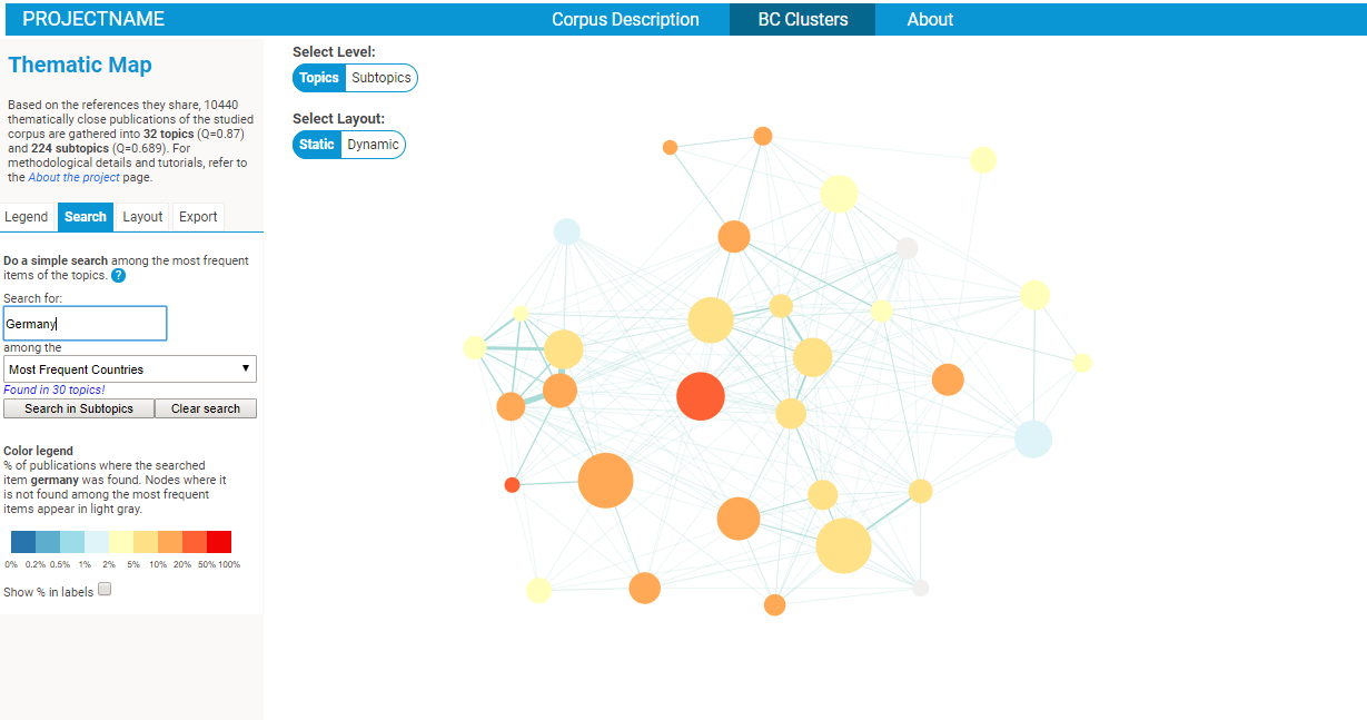
- an intuitive search functionality will allow you to quickly identify the clusters corresponding to a give ntopic / reference / etc.
- you may try to play with the spatial layout, changing some thresholds / parameters to explore the robustness of the spatial representation.
- IMPORTANT: the initial default spatial layout just put the clusters in a circle, and it does not reflect the relationships between the clusters in any meaningful way. You may want to run the "dynamic" spatial layout (option on the middle top of the interface), which you can freeze by clicking on the "START/STOP" button of the layout tab (on the left of the interface). Then, open the console in your browser's developper tools, and execute the command "outputLayout()". A pop-up will open listing the positions of the clusters (plus some other parameters) which you may copy and paste/replace" in the "data/defaultVAR.json" file. Refresh your webpage (you may need to clear your browser's stored data) and voilà! The default position is updated. Don't forget to do this for both the TOP and SUBTOP level. This manipulation may appear at bit complex, but you only have to do it once. At it will allow you to control the default position of the clusters that people visiting your website will see if and when you put it online.
Co-occurrence Maps
The command line
will create multiple co-occurence networks, all stored in gdf files that can be opened in Gephi, among which:
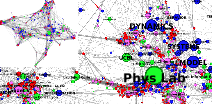
Example of heterogeneous network generated with BiblioTools and visualized in Gephi.
- a co-cocitation network, linking references that are cited in the same publications.
- a co-refsources network, linking references's sources that are cited in the same publications.
- a co-author network, linking authors that collaborated in some publications.
- a co-country network, linking countries with researchers that collaborated in some publications.
- a co-institution network, linking institutions with researchers that collaborated in some publications. For this network to be fully useful, you may want to spend some time cleaning the "institutions.dat", e.g. by keeping only the big institutions (university level) or by replacing minor name variant by the dominant name variant ("Ecole Normale Supérieure de Lyon" → "ENS Lyon")
- a co-keyword network, linking keywords being co-used in some publications. Be careful about the interpretation: keywords can be polysemic, their meaning differing from field to another (eg "model", "energy", "evolution", etc).
- an heterogeneous co-occurrence network, gathering all the items (authors, keywords, journals, subjects, references, institutions, etc), cf example on the side figure. This network will be generated only if the option "-hg" is used in the command line above.
All generated files will be stored in the "gdffiles" folder. You SHOULD edit the "cooc_graphs.py" script to adapt the different thresholds (keeping items of type x appearing in at least y publications). Keep in mind that lower thresholds mean more nodes in the network, ie a larger gdf file to handle. To choose your thresholds, you may want to have a look at the occurrence distributions in the BiblioMaps "Corpus description" interface, where you will find exactly how much items of type x appear in at least y publications. Once the gdf files are generated, upload them in Gephi and play around with Gephi's different tools (colors, sizes, filters, etc...) to produce meaningful visualizations. Refer to our Scientometrics paper for some examples!
Methodology: the weight of the co-occurrence links is defined as ωkl= nkl/√(nknl), where nkl is the number of publications where both items k and l appear and nk (resp nl) the number of publications in which k (resp l) appears. If two items never co-appear in a publication, they are not linked; if the sets of publications in which they appear are identical, the strength of their connexion is maximal (nkl=nk=nl ⇒ ωkl=1).
All analyses at once - and on multiple time periods
If you want to perform all the analyses at once, you may use the command line:
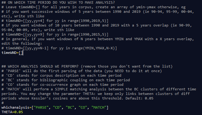
Instructions on how to edit the parameters are provided in the "all_in_once.py" script.
You may edit the parameter "whichanalysis" in the script to select the analysis you want to perform. By default, the code will:
- parse the WOS files in the rawdata folder (add the option "-d scopus" to parse Scopus data)
- perform a frequency analysis and prepare data files for the "corpus description" BiblioMaps interface.
- perform a BC analysis and prepare data files for the "BC maps" BiblioMaps interface or Gephi, + companion documents to compile in laTex. BEWARE: contrary to the biblio_coupling codes that asks you to confirm the values of some parameters along the way, the "all_in_one" script does not ask for any confirmation and always use default values.
- prepare co-occurrence graphs to be opened in Gephi.
Moreover, the "all_in_one" scripts allows you to define temporal slices on which to performs all the studies. You may for example want to perform a BC analysis on multiple 5 years periods? Just edit the "timeWND" parameter in the script before launching it on the command line: all analyses will be performed directly. To visualize the generated data files in BiblioMaps, you should follow the instructions written on the generated "AA_logs.txt" file.
Right now, the BC analysis performed on the different temporal slices are independant, although a simple analysis is performed to match clusters from one time period to clusters from the precedent / next one. More complex scripts allowing to analyse / visualize the historical evolution of BC clusters are in preparation!